How to reverse the column order in Microsoft Excel ?
This blog post will explain in simple steps on how you can flip or reverse the order of the column data in Microsoft Excel 2016.
How to reverse the column order in Microsoft Excel ?
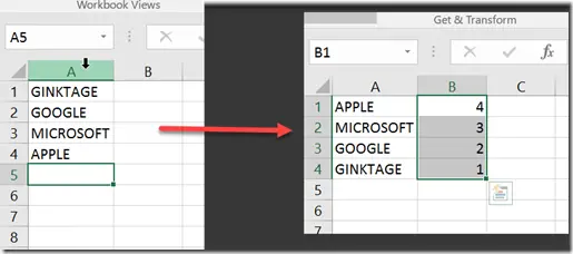
Assume that you have a data in the column A and you want to reverse the order as shown in the screenshot.
Here’s how you can do it easily using the sort command.
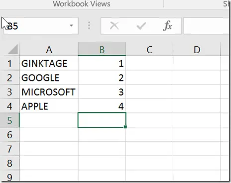
1. Insert the sequence numbers of the columns in the column B as shown.
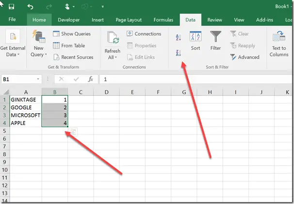
2. Select the column cells “B1 to B4” and navigate to Data Tab and select “Sort Z to A”.
3. This would display a “Sort Warning” dialog. Check the radio button “Expand the selection” and click the sort button.
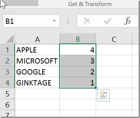
4. You will immediately notice that the order of the column A is reversed as shown in the screenshot.


Leave a Review