How to Create a Simple Drop Down list in Microsoft Excel?

This blog post will provide a step by step instruction on how you can create or insert a drop down list in Microsoft Excel 2013. This tip also works fine on other versions of Microsoft Excel like Excel 2016 and Excel 2019.

A drop down list enables the user to select the value from the predefined list instead of user typing them.

How to Create a Simple Drop Down list in Microsoft Excel 2013?

Creating a Drop Down list in Microsoft Excel is very simple and you can do that by following the below steps

When a drop down list is created, the user can enter the data by selecting it. In this blog post, I will show you how you can create a Simple Drop Down list in Microsoft Excel 2013 where the list of data to be populated comes from the same worksheet.

1. Open Microsoft Excel 2013 and create a new Excel Workbook.

2. To prepare the list of data to be populated in the Drop Down list, lets add the below data to the corresponding cells

A1 – Senthil Kumar

A2 – Senthil

A3 – Kumar

A4 – isenthil

A5 – Senthil Kumar B

3. Select the Cell where you want the drop down list to appear.

4. Navigate to the Data Tab -> Data Validation Menu and click “Data Validation” option from the dropdown.

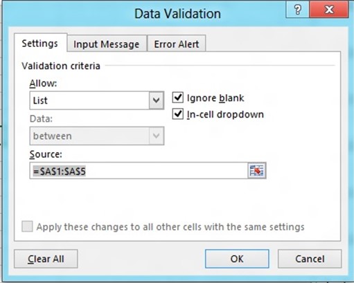
5. In the Data Validation Dialog -> Settings Tab, select “List” from the Allow option and then enter the following data in the source textbox and click OK.

=$A$1:$A$5

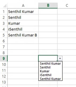
6. Now, you should see the drop down list on the selected cell.