How to Calculate Percentage in Excel Using Formula ?
Calculating percentage in Excel is one of Excel‘s most straightforward tasks if you know the formula to calculate the percentage. The percentage is nothing but an estimated value out of 100. For example, 89% means 89 out of 100.
In this article, you’ll learn how to use the percentage formula and find the percentage of a given data in Microsoft Excel.
What is the Formula of percentage in Excel ?
Microsoft Excel does not provide a direct function to calculate the percentage. Instead, it lets you use excel formulas to calculate the percentage.
How to apply Percentage Format in Excel?
To enter the percentage format in Microsoft Excel, follow the below steps
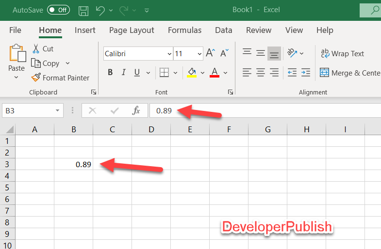
- Select a Cell (Eg : B3) and enter a decimal value 89.5
- Navigate to “Home” tab and click the percentage symbol under the “Number group” to apply the percentage format in excel.
How to Increase a Number by Percentage in Excel?
To increase a number by percentage in Excel, follow the below steps.
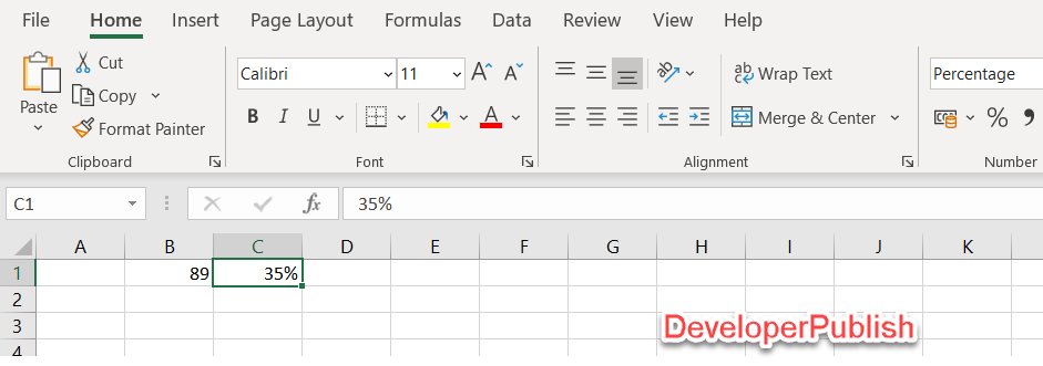
- Enter a number (Eg : 89) in cell B1. Enter a decimal number (0.35) in cell C1 to indicate that you want to increase the number in BE by 35% and then apply a Percentage format for the cell C1.
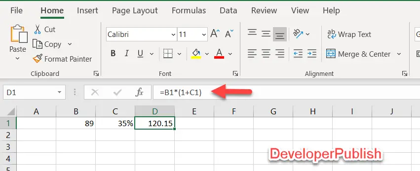
- To increase the number in cell B1 by 35%, multiply the number by 1.35 (1+1.35). Select the cell D1 and enter the following formula =B1*(1+C1)
How to Calculate the Percentage of Change between Numbers in Excel?
To calculate the percentage of change between numbers in Excel, follow the below steps
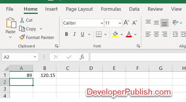
- Enter the first number in cell A1 and the second number in cell B1.
- Apply the formula =(B1-A1)/A1 for the cell C1. This formula calculates the the difference between first and the second number. Then divide this result by the first number (Cell A1).
Advanced Percentage Calculation in Excel Using Formula
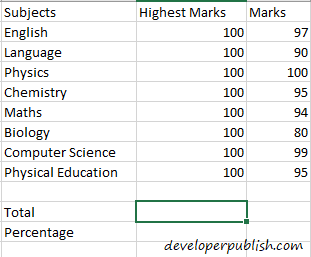
To show an more advanced percentage calculation , lets have a look at student’s marks sheet and show the total percentage of marks that the student has got out of all subjects.
- Assume that the student has got the marks for the subjects as shown below.
- To calculate a percentage first you need to find the total. So we use the SUM function to calculate the total of the marks and the marks obtained by the student and display the result in the cell F11.
- Select the SUM function to find the total.
- Enter the range of the cells which contain the marks that should be summed up. Click on OK to proceed.
- Then you get the total of the marks of all the subjects. Similarly, calculate the sum of the marks obtained by the student.
Now let’s proceed to how to find the percentage.
- To find the percentage of the total marks you need the total which is then divided by the total marks in this case and then multiplied by 100.
- So go to the formula bar enter the formula, in this case, =SUM(F2:F9)/800*100 to calculate the highest percentage and similarly =SUM(G2:G9)/800*100 to find the percentage of the marks obtained by the student.
- Here we use previously calculated sum i.e, total instead of using the SUM function again.
Similarly use the formula =G11/800*100 to calculate the percentage obtained by the student. Here we use G11 which is the total scored by the student which is divided by the total highest mark i.e, 800 which is in the cell F11, and then multiplied by 100.





Leave a Review