Format Cells in Microsoft Excel

In this article, you’ll get to know about formatting cells and how to use them in Microsoft Excel.

What is the formatting of cells?

Formatting in common is making changes to display data in more preferable way.

Similarly in Microsoft Excel formatting of cells means changing its properties such as its alignment, the default font style, font size, font color, cell border, cell color, cell format, and its protection to your convenience. Formatting a cell does not affect the data it contains.

It only changes the outlook or the way it gets displayed.

How to format cells in Excel?

To format cells in a worksheet, to your wish do the following steps.

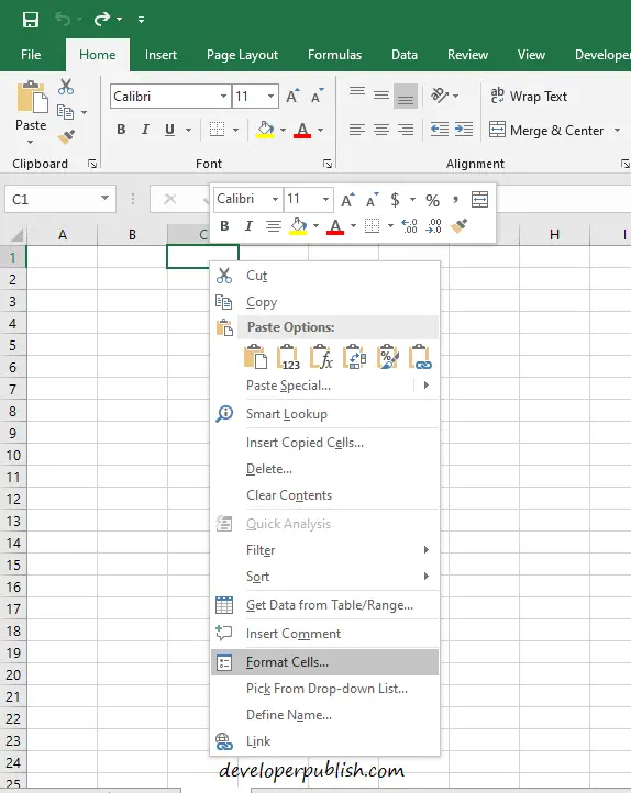
• Select a cell in the worksheet.

• Right-click on the cell.

• Select Format Cells from the list of options that are displayed.

Tip: You can also use the control keys Ctrl+1 to go to the Format dialog box instead of performing the right click action.

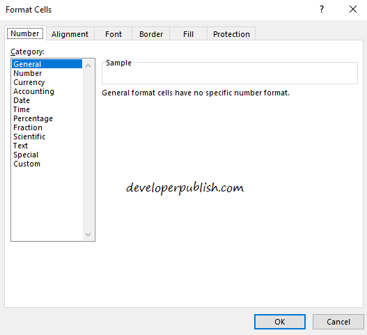
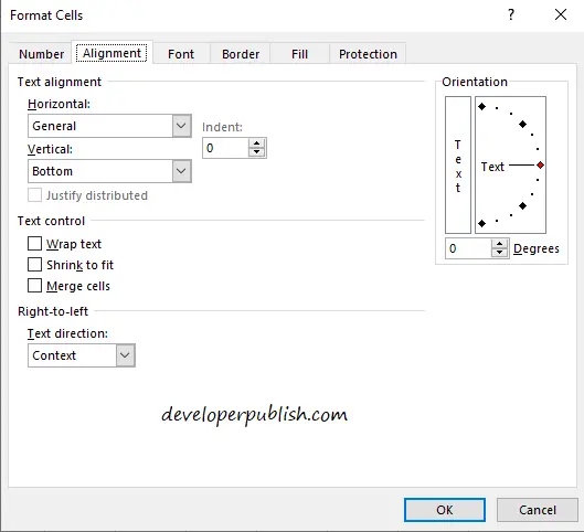
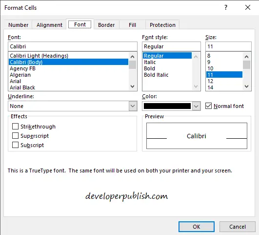
• When the Format dialog box opens up you can select what changes you want to make. It has six tabs i.e, Number, Alignment, Font, Border, Fill, Protection.

• Under Number, you’ll find options to change the number format of the cell.

• Under Alignment, you have options to change the text alignment, text orientation, its direction of flow, and its fit.

• Then in Font, you can change the font type, font style, font color, font size, underline, or non, and you can also choose between special effects such as strikethrough, subscript, and superscript.

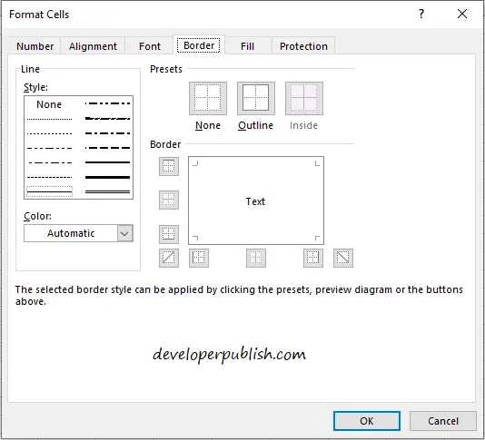
• In Border, you can fix the border of the cell, its color, and its style. You can also choose a preset that is already provided by Excel.

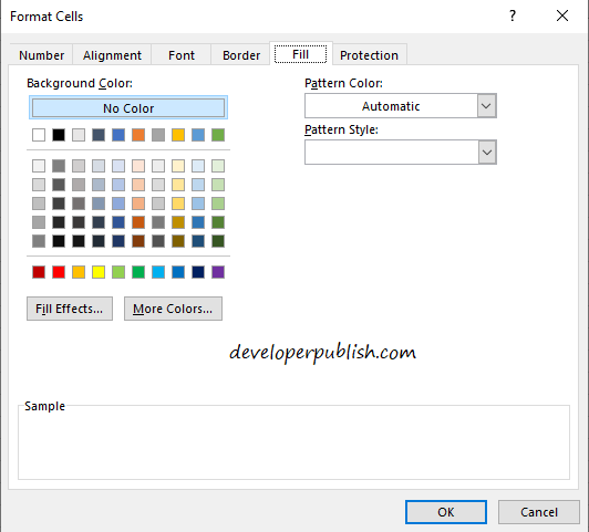
• In Fill, you can choose your cell color or set a set pattern to the cell and also choose the color of the pattern.

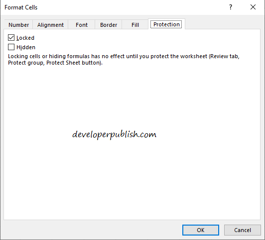
And finally the under Protection, you have the option to either hide the cell or lock the cell. However, these options are effective only if your worksheet is protected.

We hope you understood the concept of formatting in Microsoft Excel.