COMBINA function in Excel
In this post, you will learn about the COMBINA function in Excel and how it is used in-with excel spreadsheets.
COMBINA function in Excel
- The Function returns a number of combinations for a given number of items.
- For example, consider the following numbers 1,2,3 .We have a total of 3 numbers and we want to group them in 2’s.
With the given data the combinations are as follows
| 1, 1 | 1, 2 | 1, 3 | 2, 2 | 2, 3 | 3, 3 |
Hence the total number of combinations 6 is your answer
- This function allows repetitions when it creates the combinations, which makes it different from the Combin function.
- Note: The Combin function is another type of combination function which does not allow repetition.
Syntax
=COMBINA(number, number_chosen)
The Syntax has two arguments:
number – This holds the total number of the group of data characters/numerals to be used in the function.
The number used in this argument should be greater than or equal to 0 and it should also be greater than the value used in the second argument (number_chosen)
number_chosen – The argument holds the value of how the characters or numerals are to be grouped.
The number used in this argument should be greater than or equal to 0.
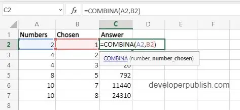
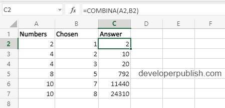
How to use COMBINA Function in Excel?
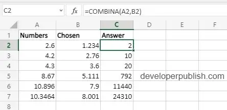
The example below uses decimal numbers. When inserted in the function they are shortened into integers, that is they do not affect the function in any way.
Additional Points:
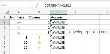
- Both the arguments are required to perform the function, and mostly integers can be used. The syntax does not accept non-numeric values and returns #VALUE!.
- You can use decimal numbers in this function as it shortens them into integers.
- It is important that you know that the numbers used in the function are the total count and not the data.


Leave a Review