CEILING.PRECISE Function in Excel
In this post you will learn about the Ceiling.precise Function in Excel. This Function has a similar working as the Ceiling Function, it rounds up the number to the nearest high value and hence the name Ceiling.
CEILING.PRECISE Function in Excel
Syntax
=CEILING.PRECISE(number, significance)
Arguments
The syntax of the Ceiling function has two arguments
- number – The number you want to round up
- significance – The multiple to which you want to round the number, default value is 1.
- The arguments in syntax can have be an integer or a decimal numbers.
- Note that the number is rounded up to the nearest significance value multiples and not the number itself; Example =CEILING.PRECISE(5, 3) answer is 9 a multiple of 3.
- The significance argument is optional as it has a default value.
How to use Ceiling.precise function in Excel?
- This function rounds up the number towards the nearest integer or the multiple of the given significance.
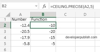
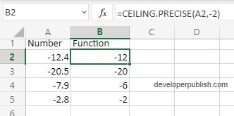
- For negative numbers this function always rounds up the number towards zero, as it does not consider the the sign of the significance argument.
Examples:
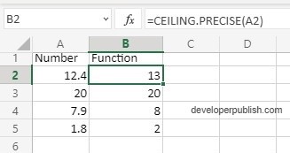
In the following example the Ceiling.precise function works with the default significance argument value (1).
When the significance value is 1, the function sometimes returns the number unchanged this is happens when there is no need to round up the number as it satisfies the significance value.
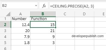
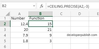
In the examples below the Ceiling.precise function syntax has:
- Positive number and positive significance argument value (3)
- Positive number and negative significance argument value (-3)
- Negative number and positive significance argument value (5)
- Negative number and negative significance argument value (-2)



Leave a Review