Index and Match in Microsoft Excel
This post explains the Index and Match function in Excel and also the various lookup types available in Microsoft Excel.
Index in Excel
The Index function in Excel simply returns the specific value from a range of cells by reference to the given location.
=INDEX(lookup_array, row_no, [column_no])
Example
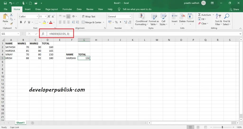
=INDEX(D2:D5, 3)
When you select a particular range, the first cell in that range will denote row_number 1. So here D4 will be denoted by 3 as row number.
Match in Excel
In Microsoft Excel, you can locate the position of a particular value in a column, row, or table by using the Match function.
=MATCH(lookup_value, lookup_array, [match_type])
Match function supports both approximate and exact match types.
Example
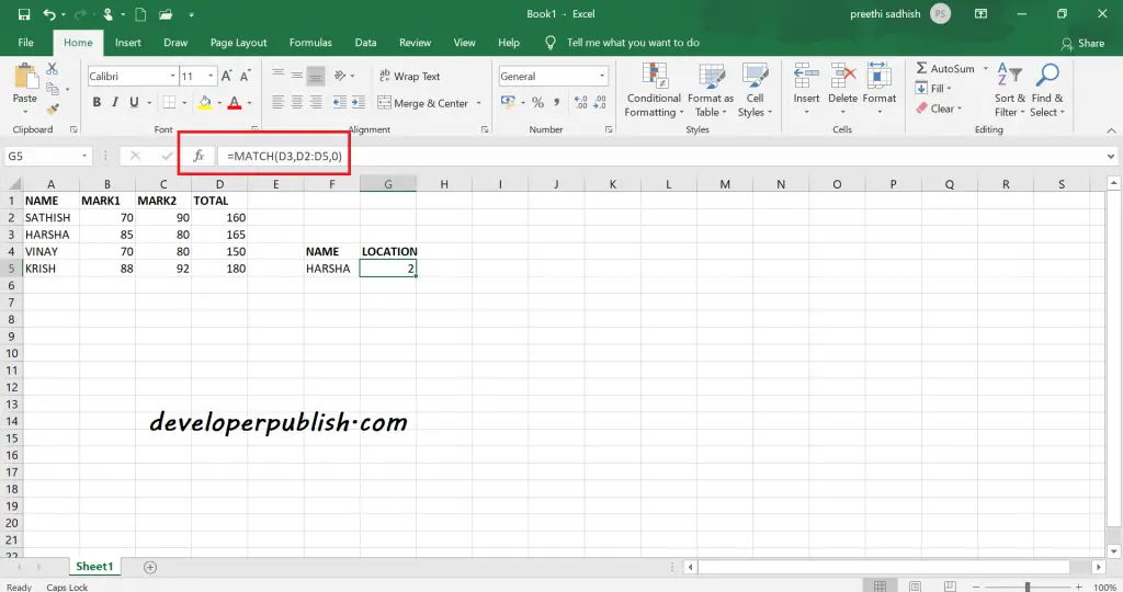
=MATCH(D3, D2:D5, 0)
Index and Match in Excel
In many cases, the Match function combines with the Index function to retrieve a value at a matched position.
As you know the Match function returns the location of the value, so this can be used inside the Index function to find the value in that particular location.
=INDEX(lookup_array, MATCH(lookup_value, lookup_array, [match_type]))
Example
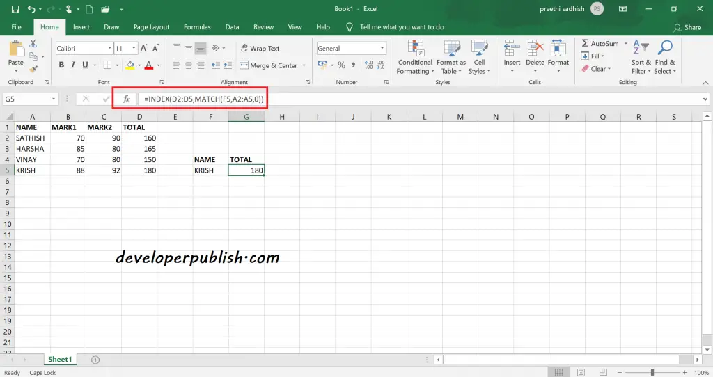
=INDEX(D2:D5, MATCH(F5,A2:A5,0))
Two-way Lookup in Excel
Using the Index and Match function you can get a value from a two-dimensional range. This is the Two-way Lookup.
Here use two match functions along with the index function.
=INDEX(lookup_array, MATCH(….), MATCH(….))
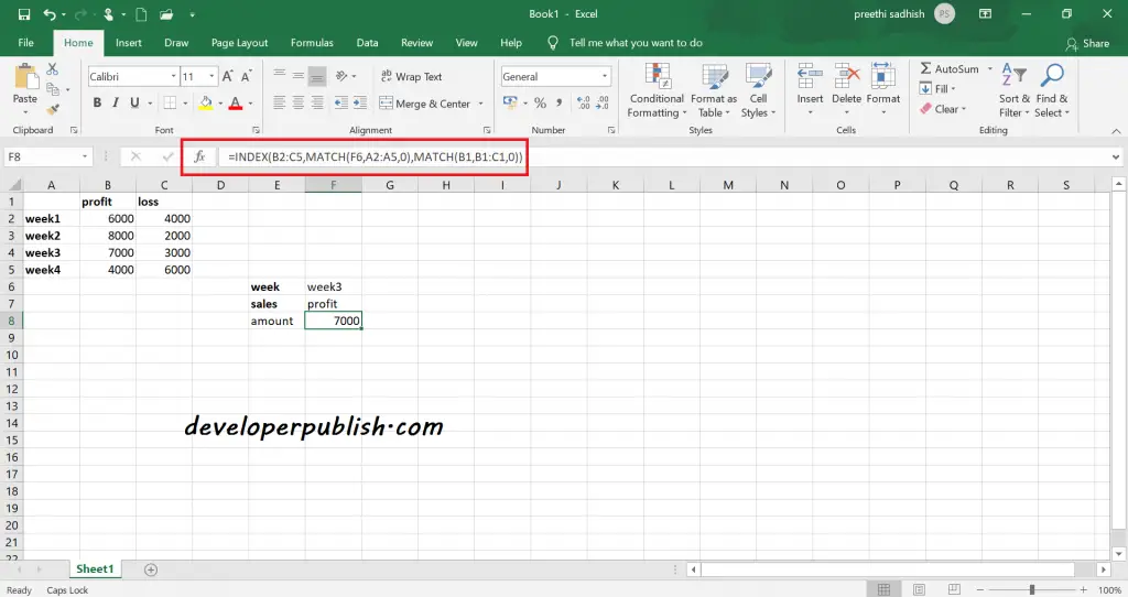
Example =INDEX(B2:C5,MATCH(F6,A2:A5,0),MATCH(B1,B1:C1,0))
Case-Sensitive Lookup in Excel
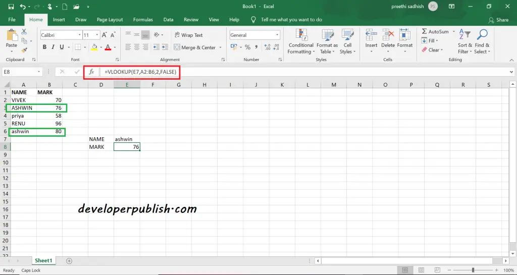
The Vlookup function in excel performs a case-insensitive lookup by default. So you can use the Index, Match, and Exact to perform a case-sensitive function.
=INDEX(lookup_range(MATCH(TRUE,EXACT(lookup_value, range),0))
Example
Since Vlookup is case-insensitive it returns ASHWIN’s value instead of ashwin. You can overcome this by the below functions.
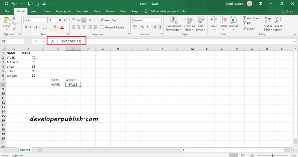
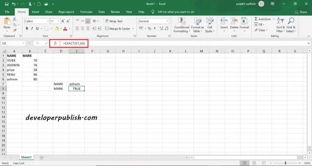
Here the Exact function performs as shown below
=EXACT(E7,A3)
Returns True if it finds the exact match and False when there is no exact match.
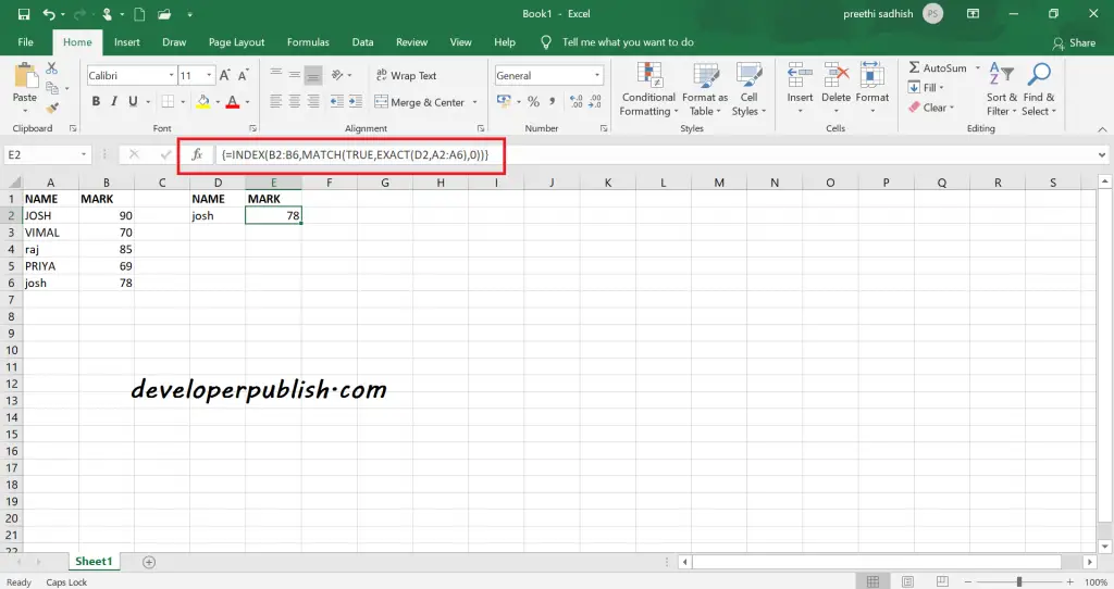
Now, this Exact function is used in the Index function to perform a case-sensitive operation.
=INDEX(B2:B6,MATCH(TRUE,EXACT(D2,A2:A6),0))
Left Lookup in Excel
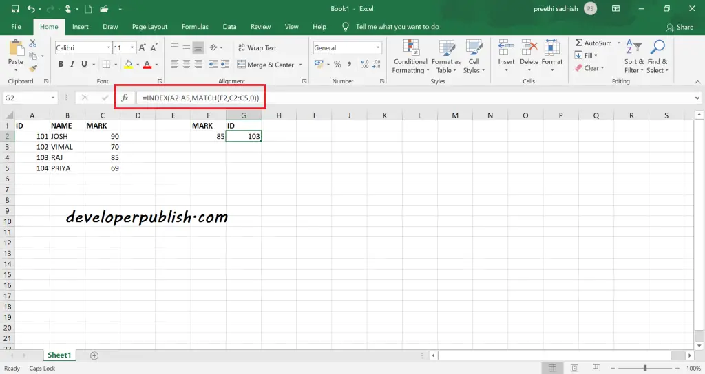
In Microsoft Excel, the VLOOKUP function only looks to the right. The left lookup can be done using INDEX and MATCH.
=INDEX(lookup_array, MATCH(lookup_value, lookup_array, [match_type]))
Example : =INDEX(A2:A5,MATCH(F2,C2:C5,0))
Two-column Lookup in Excel
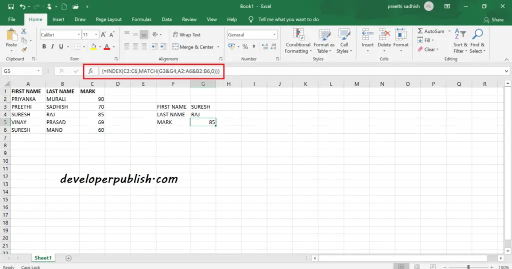
Using the Index and Match function you can look up a value on multiple criteria.
=INDEX(range, MATCH(value1&value2,range1&range2,0))
Example : =INDEX(C2:C6,MATCH(G3&G4,A2:A6&B2:B6,0))
Closest Match in Excel
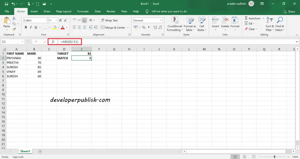
Using Index, Match, ABS, and Min you can find the closest match to the target value in a range.
=INDEX(range, MATCH(MIN(ABS(range – lookup_value)), ABS(range – lookup_value))
The ABS calculates the differences between the target value and the values in the data column.
=ABS(range values – target value)
Example
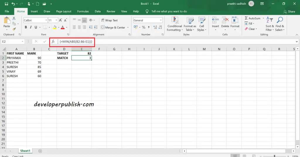
The MIN function finds the minimum value among the ABS range.
=MIN(ABS(range values – target value)
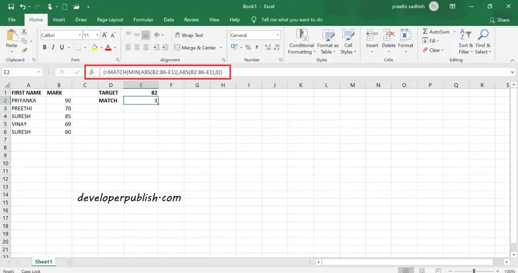
The MATCH function retrieves the position of the minimum value found using the MIN function.
=MATCH(MIN(ABS(range values – target value)
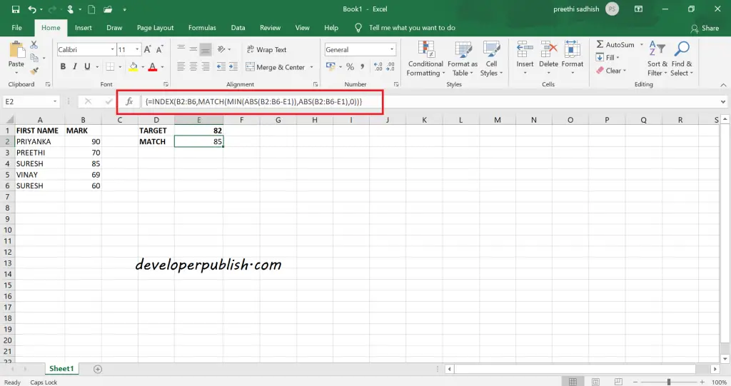
Finally, the INDEX function returns the closest value of the target value from the range.
=INDEX(B2:B6,MATCH(MIN(ABS(B2:B6-E1)),ABS(B2:B6-E1),0))



Leave a Review