How to create drop down list in Excel to use data from other worksheet ?
In one of my previous blog posts, I showed How to Create a Simple Drop Down list in Microsoft Excel 2013 using the data from the same worksheet.
In this blog post, I will demonstrate how one could create a Drop Down list in Microsoft Excel 2013 to use data from a different worksheet.
How to create a drop-down list in Excel to use data from other worksheets?
1. Let’s enter the following data in the worksheet 1
A1 – Senthil Kumar
A2 – Senthil
A3 – Kumar
A4 – isenthil
A5 – Senthil Kumar B
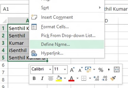
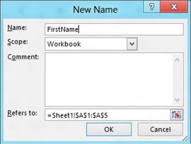
2. Drag the Cells A1 to A5 and right click and then select “Define Name” from the context menu. Let’s provide the name “First Name” to it and click OK.
3. Now, go to the Worksheet 2 and select the cell/column where you want the drop-down list to be shown and then click the Data Tab.
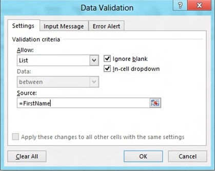
- Navigate to Data Validation Dialog by clicking the Data Validation button from the Data Validation combo box defined in the Data Tools.
- In the Settings Tab, select the option “List” in the Allow Drop down and in the Source text box, enter =FirstName and click OK.
6. You should now see the drop-down list created in the selected column of the excel worksheet 2 with the predefined values from worksheet1.


Leave a Review