DELTA Function in Excel

In this article, you will learn about the DELTA function, the formula syntax and usage of the function in Microsoft Excel.

DELTA Function in Excel

The delta function in Excel compares two numeric values and when equal the function returns 1 and if not it returns a 0.

Syntax 

=DELTA (number1, [number2])

Arguments 

• number1 – The first number.
• number2 – [optional] The second number.

Possible Errors

• When the first argument ‘number1’ is nonnumeric, DELTA returns the #VALUE! error value.
• If number2 is nonnumeric, the function returns the #VALUE! error value.
• When the number2 is left blank, DELTA assumes number2 equals zero.
• And if either value of the arguments is text, DELTA returns the #VALUE error.

How to use DELTA function in Excel Worksheet?

Using this function in a WS is simple; all you need to do is enter the function as a formula of the cell in the formula bar.

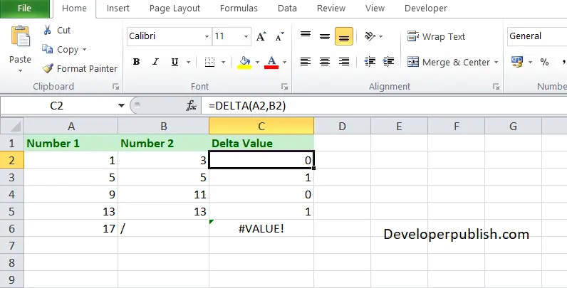
Take a look at the given example

To find the DELTA value between two numbers, Enter the given numbers in column A and column B, enter the following formula in column C,

Formula: =DELTA (A1, B1)

Here, A1 and B1 refer to the cell name or the cell address. Repeat the same to the other cells and you will get the DELTA of the two numbers.

From Cell A6 and B6, you can find that the corresponding value is #VALUE! error, that is due to the presence of non-numeric characters.