3D reference in Excel
In this post, let’s learn about 3D reference in Excel. 3D reference in Microsoft Excel is like working on the same cell in different worksheets at the same time.
How to use 3D reference in Excel?
This method is simple and effective. When you wanna refer to the same cell but from different worksheets just use this format of the function =funtion(First sheet:last sheet!cell reference).
Lets take a look at a example.
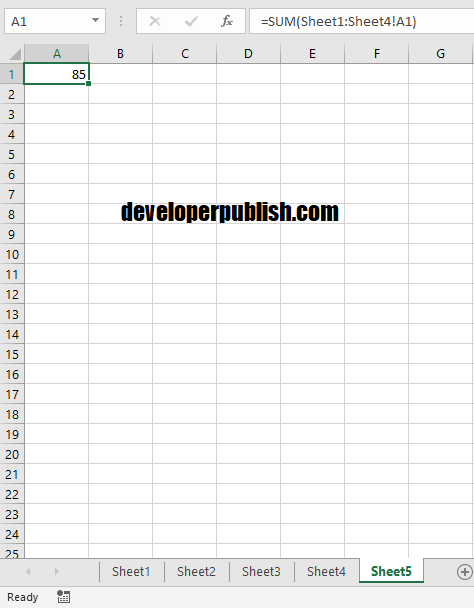
For instance you wanna sum up the values in A1 from the first four worksheets. You can use the function as SUM(Sheet1:Sheet4!A1)
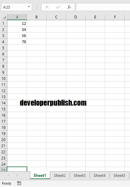
The first sheet has these values.
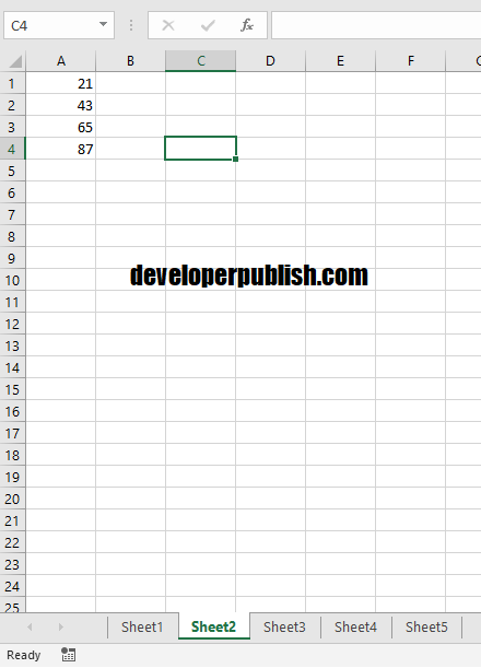
The second sheet has these values.
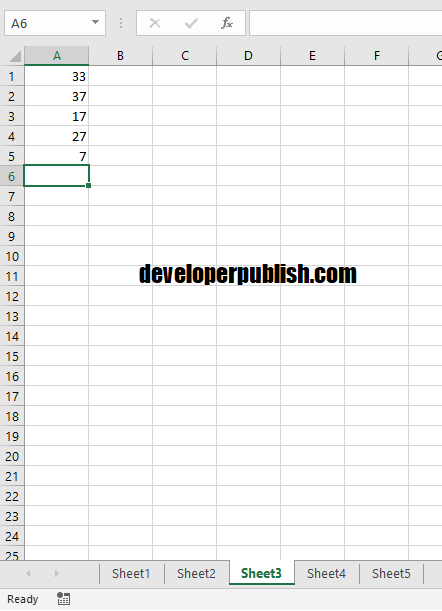
The third sheet has these values.
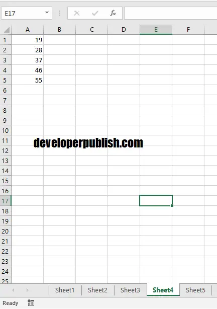
The fourth sheet has these values.
Now in the fifth sheet when you enter the function SUM(Sheet1:Sheet4!A1) in the formula bar, you can see the result.
That is all about 3D reference in Excel.



Thanks for teaching me how to use the 3D reference in Excel.