SKEW Function in Excel

In this article, you will learn about the SKEW function, the formula syntax and usage of the function in Microsoft Excel.

SKEW Function in Excel

The SKEW function in Excel returns the skewness of a distribution, which is a measure of symmetry. A positive result indicates distributions that extend towards the right. A negative result indicates a distribution that extends towards the left. 

Syntax

SKEW(number1, [number2], ...)

Arguments:

• Number1, number2, …    Number1 is required, Other subsequent numbers are optional.

The argument can range from 1 to 255 arguments for which you want to calculate skewness.

You can also use a single array or a reference to an array instead of arguments separated by commas.

Possible Errors and usage notes

• Arguments can either be numbers or names, arrays, or references that contain numbers.
• Logical values and text representations of numbers that you enter are counted.
• When an array or reference argument contains text, logical values, or empty cells, those values are ignored; however, cells with the value zero are included.
• In case of  there are fewer than three data points, or the sample standard deviation is zero, the SKEW function returns the #DIV/0! error value.
• The equation for skewness is defined as:

 How to use the SKEW function in Excel?

Using this function in a WS is simple; all you need to do is enter the function as a formula of the cell in the formula bar.

Take a look at the given example

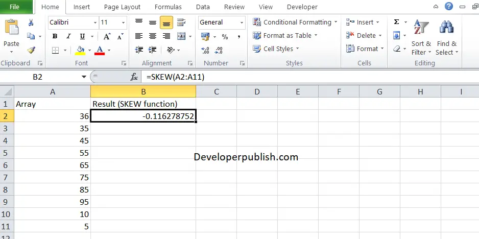
Enter the data in the respective columns and enter the SKEWfunction formula.

Formula: =SKEW(A2:A11)

Here, A2 refers to the cell name or the cell address. Column A denotes the Array.