Lookup and Reference Functions in Microsoft Excel
This post is about the Lookup and Reference Functions in Microsoft Excel and how you can use these functions effectively.
Lookup and Reference Functions in Microsoft Excel
Lookup & Reference functions help you work with different data sets and are useful in cross-checking the data. Using these functions, you can get information about a range of data, the location of a given value, or look up for specific values.
Here let us check out some of the Lookup and Reference functions with examples:
VLOOKUP
The VLOOKUP (i.e, Vertical Lookup) function finds a value in the table’s leftmost column. It then displays the value in the same row from another column you specify.
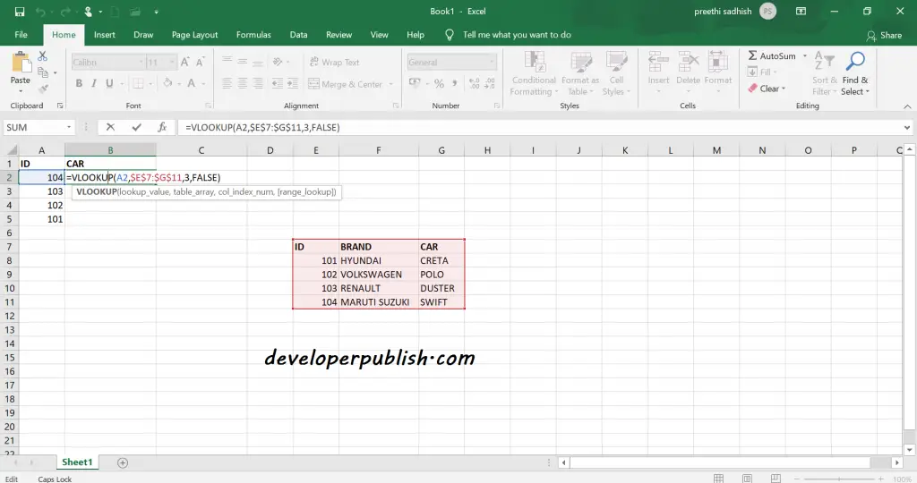
- In the cell where you want to get the value, insert the VLOOKUP function.
=VLOOKUP(A2,$E$7:$G$11,3,FALSE)
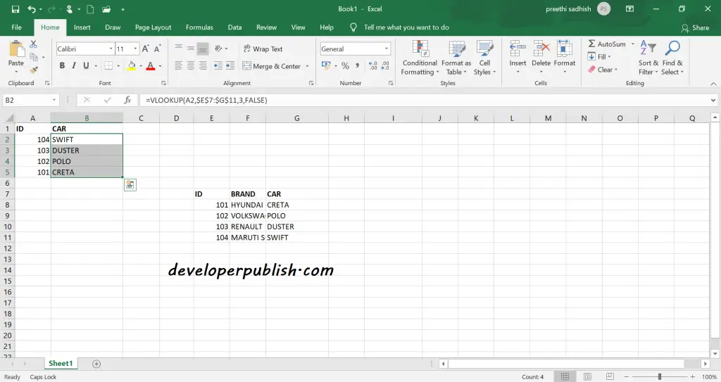
the VLOOKUP function looks for the ID 104(A2) from the range ($E$7:$G$11) and returns the value from the third column(3). The argument FALSE is set to return an exact match or a #N/A error if not found.
- Drag the VLOOKUP function in cell B2 down to cell B5 so the cells below will be automatically updated.
HLOOKUP
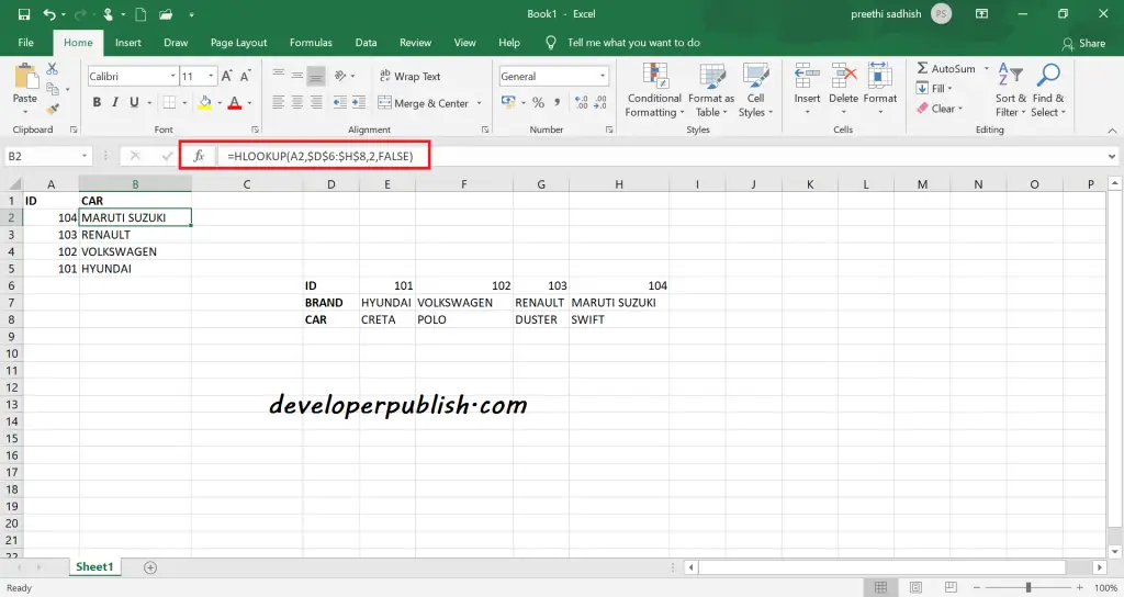
The HLOOKUP (horizontal lookup) function searches for a value in the top row of a table and then returns a value in the same column from a row you specify in the table.
=HLOOKUP(A2,$E$6:$H$8,3,FALSE)
MATCH
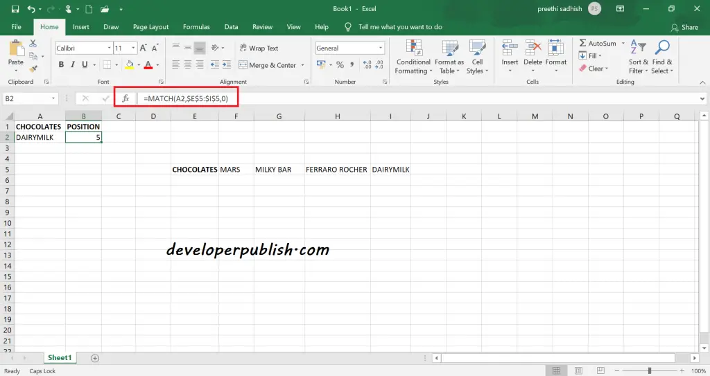
The MATCH function returns the position of a value in a given range.
=MATCH(A2,$E$5:$I$5,0)
Here the fourth argument indicates:
- 0 -> exact equal
- 1 -> less than
- -1 -> greater than
INDEX
Uses an index to choose a value from an array.
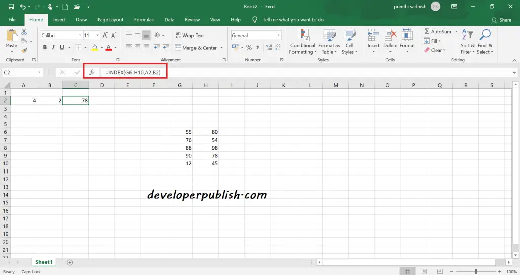
=INDEX(G6:H10,A2,B2)
Here G6:H10 is the array to be looked upon, A2 and B2 are the row number and column number respectively.
CHOOSE
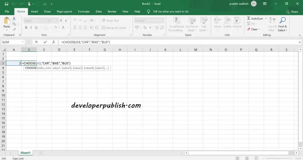
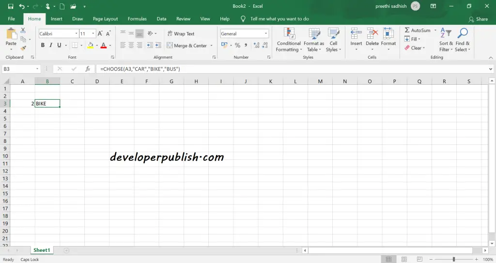
The CHOOSE function returns a value from a list of values, based on a position number.
A3 is the index number and the rest is the list of values the user gives.



Leave a Review