Hide and lock formulas in Excel

This post tells about the usage of the hide and lock formula feature available in Microsoft Excel and how you can unprotect and unhide the same.

How to Lock formulas in Excel ?

When we go through a worksheet full of formulas there are chances of editing the formula accidentally, this may result in a huge error.

So here Excel allows the user to protect the cells with formula alone, instead of protecting the entire worksheet.

To lock formulas in Excel firstly you need to unlock all cells in the worksheet, to do so follow the below steps:

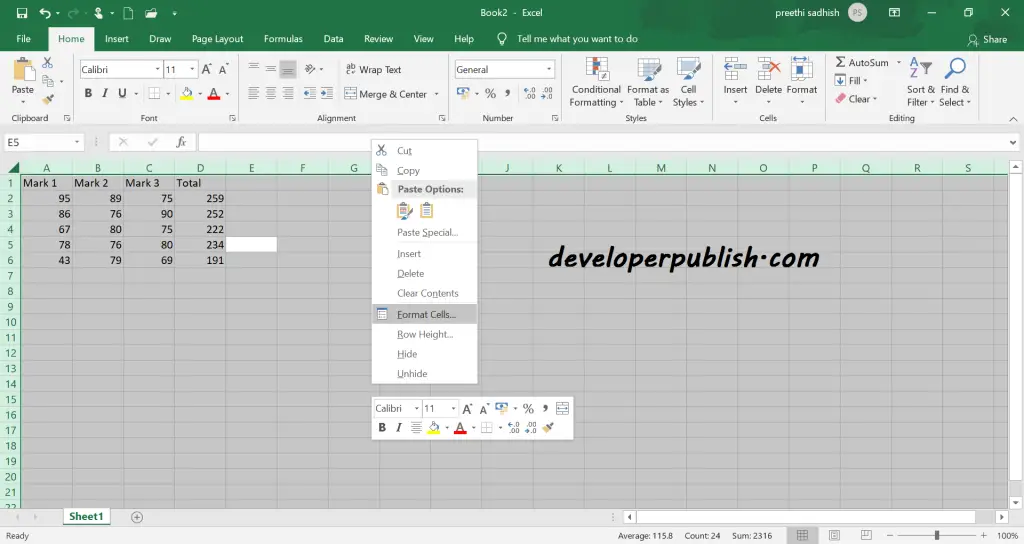
• Select all cells in the worksheet by pressing Ctrl+A.

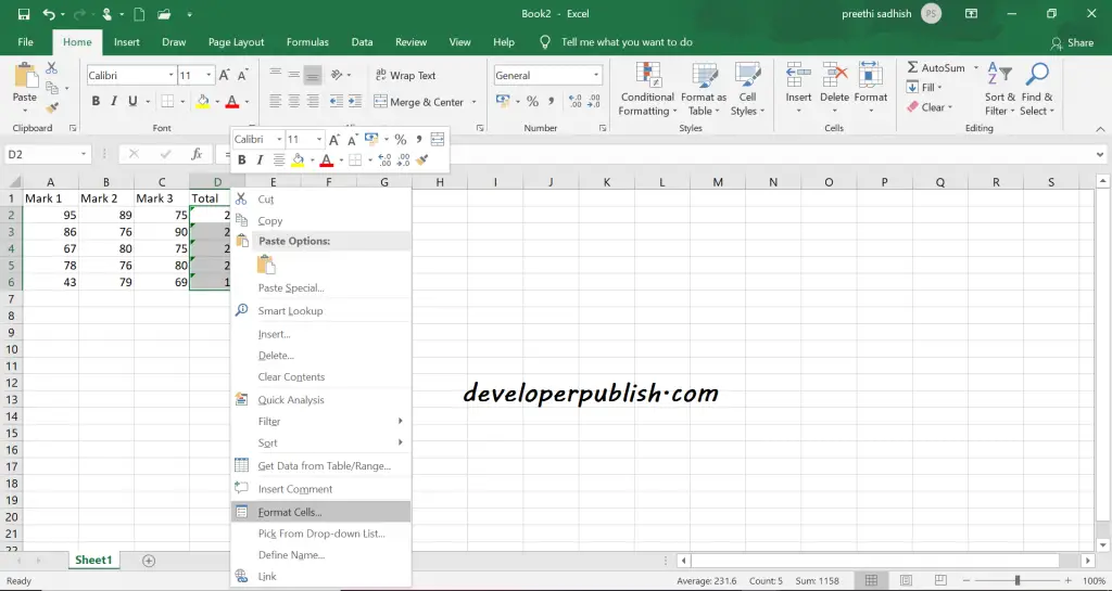
• Right Click and select Format cells or press Ctrl+1.

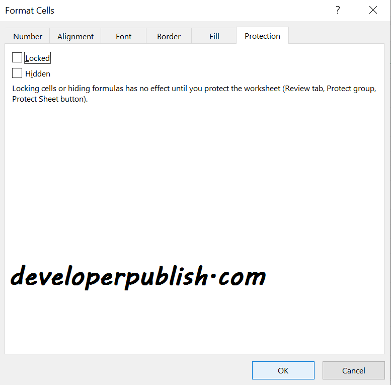
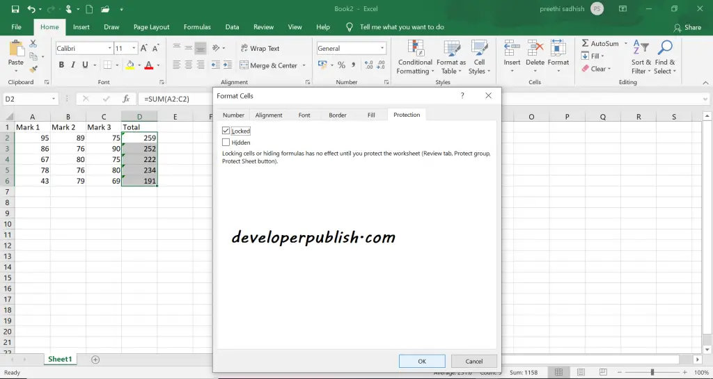
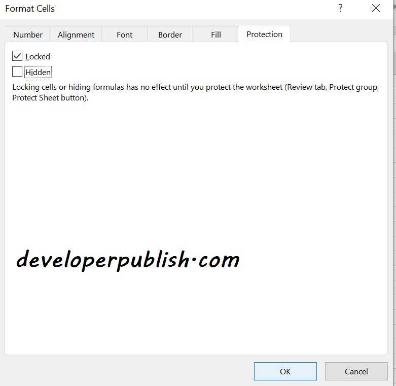
• Select the Protection tab from the format cells dialog box.

• Uncheck the locked option.

• Click OK.

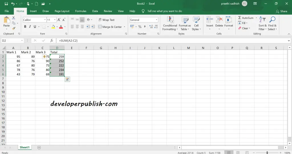
Now you have to identify and select the cells with the formula:

• Select all cells in the worksheet by pressing Ctrl+A.

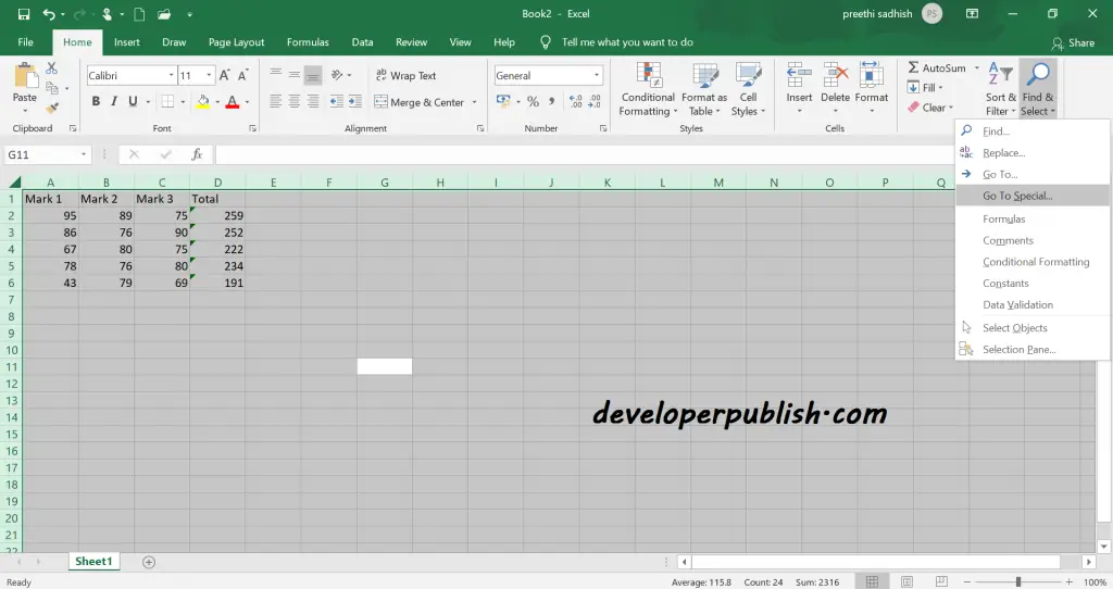
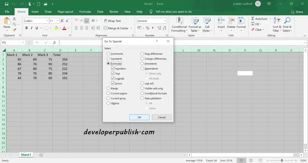
• Go to the Home tab and then click on Find & Select from the editing group.

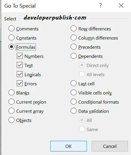
• A drop-down appears, select Go to special, and then select formulas.

• Click OK.

Now the cells with formulas will be automatically selected.

Once done,  you have to lock the cells with the formula.

Below are the steps to follow:

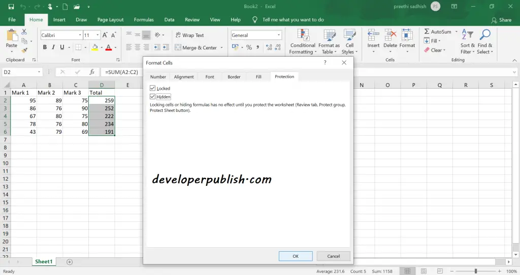
• With the cells with formula selected, Right Click and select Format cells or press Ctrl+1.

• Select the Protection tab from the format cells dialog box.

• Check the locked option.

• Click OK.

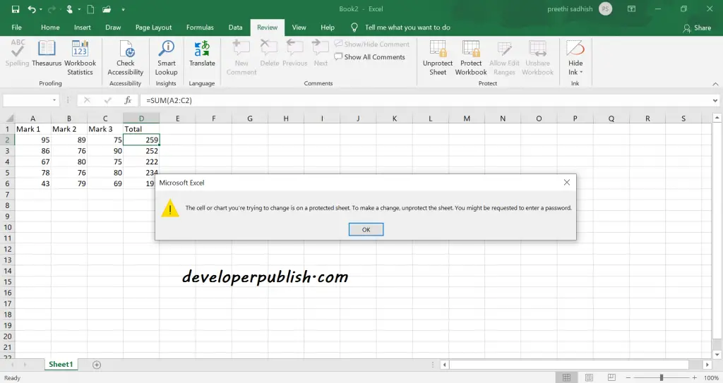
The lock cells with formula would be complete only when you protect the worksheet.

Follow the given steps:

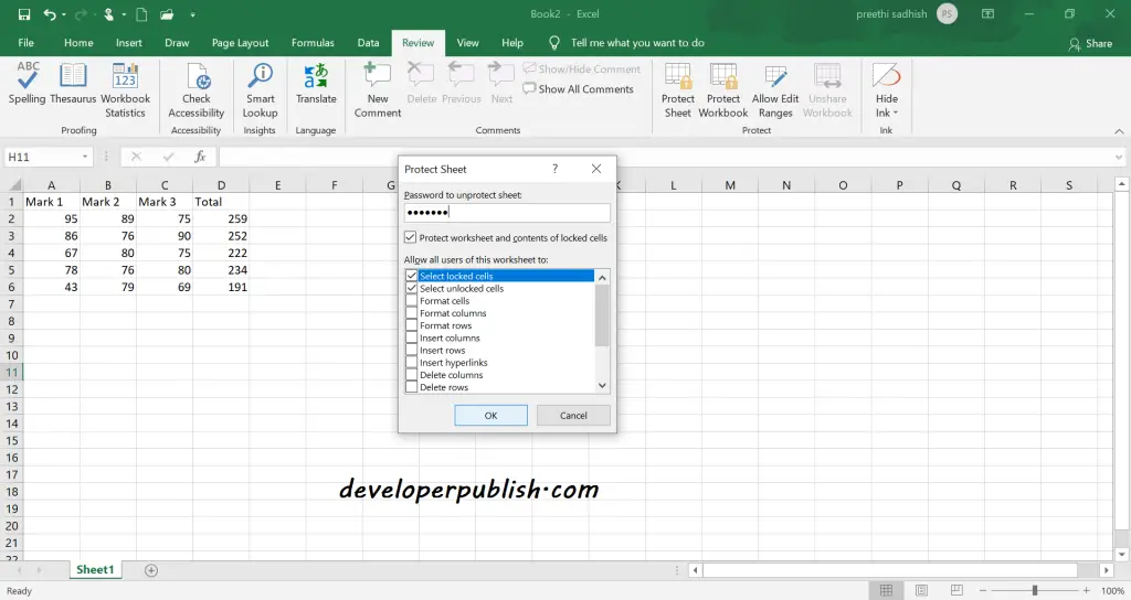
• Select the Review tab and click on the Protect sheet.

• A dialog box appears, make sure to check the ‘Protect worksheet and contents of the locked cells’.

• Specify the password and reenter the password.

• Click OK.

Finally, the cells with the formula are locked and the users cannot change anything with the formula.

How to Hide Formulas in Microsoft Excel ?

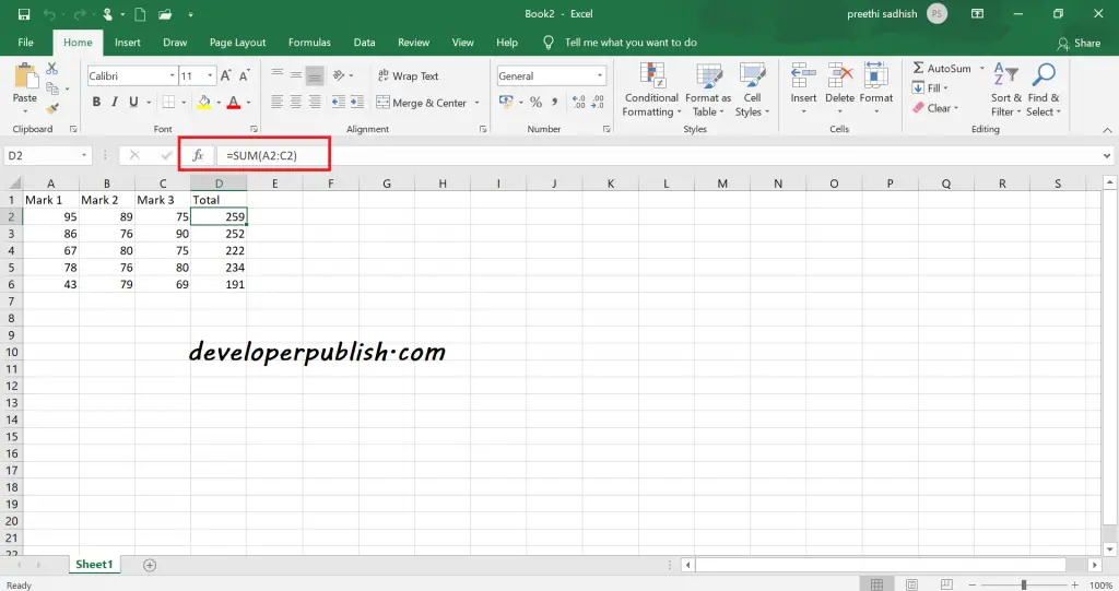
Locking the formula cells will not allow the users to edit but the formula will be visible in the formula bar.

Excel provides an option to hide the formulas also. The steps to hide formulas in locked cells:

• Select all the cells in the worksheet using Control + A.

• Go to Home and click on Find & Select from the Editing group.

• A drop-down appears, select Go to special, and then select formulas

• Click OK.

Now the cells that have formulas will be selected.

• Right-click and select Format cells or Press Control + 1. This will open the format cells dialog box.

• In the Format Cells dialog box, select the Protection tab.

• Check the Hidden option.

• Click OK.

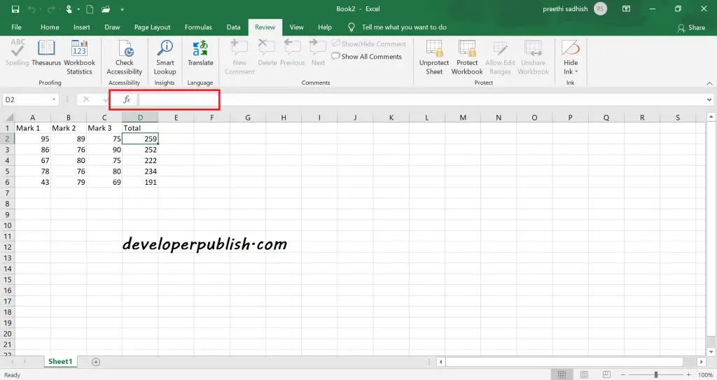
Now, if the user selects a cell with a formula and is locked, he/she will not be able to see the formula in the formula bar.

How to unprotect and unhide formulas in Excel?

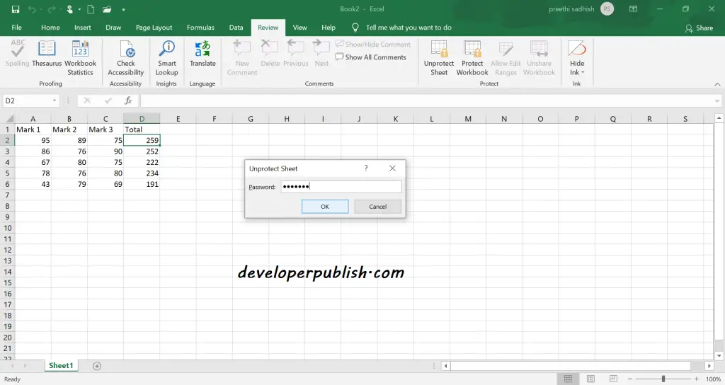
• Go to the Review tab and select Unprotect sheet.
• Enter the password and click OK.

You may want to uncheck the Hidden checkbox after unprotecting the worksheet to let the users see the formulas for future use. Press Ctrl + 1 to open the Format Cells dialog box, go to the Protection tab and uncheck the Hidden box.