In this article, you will learn about the XIRR function, the formula syntax and usage of the function in Microsoft Excel.
XIRR Function in Excel
The XIRR function in Excel is a financial function. It returns the internal rate of return (IRR) for a series of cash flows that occur at irregular intervals.
Syntax
=XIRR (values, dates, [guess])
Arguments
- Values – Array or reference to cells that contain cash flows
- Dates – Dates that correspond to cash flows
- guess [optional] – An estimate for expected IRR (Default is .1 (10%))
Possible Errors and Usage Notes:
- As we know Excel stores dates as sequential series of numbers, i.e., January 1, 1900 is serial number 1, and January 1, 2008 is serial number 39448 as it is 39,448 days after January 1, 1900.
- Numbers in dates are truncated to integers.
- The function XIRR expects at least one positive cash flow and one negative cash flow; otherwise, XIRR returns the #NUM! error value.
- In case of the date is not a valid date, XIRR returns the #VALUE! error value.
- If the given date precedes the starting date, XIRR returns the #NUM! error value.
- If values and dates contain a different number of values, XIRR returns the #NUM! error value.
- In most cases you do not need to provide guess for the XIRR calculation. If omitted, guess is assumed to be 0.1 (10 percent).
- XIRR function in Excel is closely related to the XNPV excel function commonly known as the net present value function.
- The rate of return calculated by XIRR is the interest rate corresponding to XNPV = 0.
- Excel uses an iterative technique for calculating the rate of return. Using a changing rate, XIRR cycles through the calculation until the result is accurate within 0.000001 percent.
- If XIRR can’t find a result that works after 100 tries, the #NUM! Error value is returned.
- The rate is changed until:

where:
- di = the ith, or last, payment date.
- d1 = the 0th payment date.
- Pi = the ith, or last, payment.
Example using XIRR function in Excel
Take a look at the table below:
| Values | Dates |
| -5000 | 06-Sep-99 |
| 7000 | 20-Jul-2000 |
| 2500 | 15-Feb-09 |
| 4750 | 1-Apr-09 |
| 3500 | 30-Oct-08 |
Formula: =XIRR(A2:A6, B2:B6, 0.1)
Enter the Values in Column A and Dates in Column B, and the XIRR calculation value is 0.1 by default. Now enter the formula in C1, you will get the rate of return.
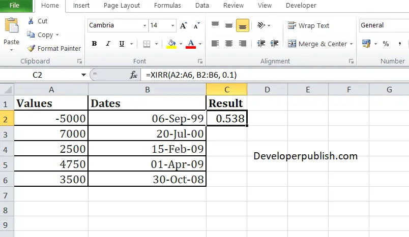
Result:
The internal rate of return is 0.538 or 53.8%.