This blog post will provide you a simple tip on how to use Custom Cell Formatting in Microsoft Excel 2016 to display a number in 4 digits.
Assume a scenario where you have a ID column in your excel sheet and you want it to have a consistent format like 0001 , 0002 instead of 1 , 2 etc.
Well , you can go ahead and type 0001 etc… but how about formatting the cell such a way that when you enter 1 , it automatically converts that to 0001 ?. Here’s how we do it.
1. Open your worksheet in Microsoft Excel.
2. Right Click on the column or cell and select “Format Cells” in the context menu.
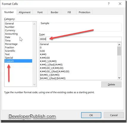
3. In the Format Cells Dialog , select the “Number tab”. You will notice that apart from the general built-in types like General,Number,Currency,Accounting etc , there are 2 more categories that are unique : Special and Custom. The special category is used for phone numbers , postal codes etc. where as the Custom category is used for creating our own formatting pattern. Select “Custom” category from the left side bar and enter 0000 in the Type textbox as shown in the screenshot and click the OK button.
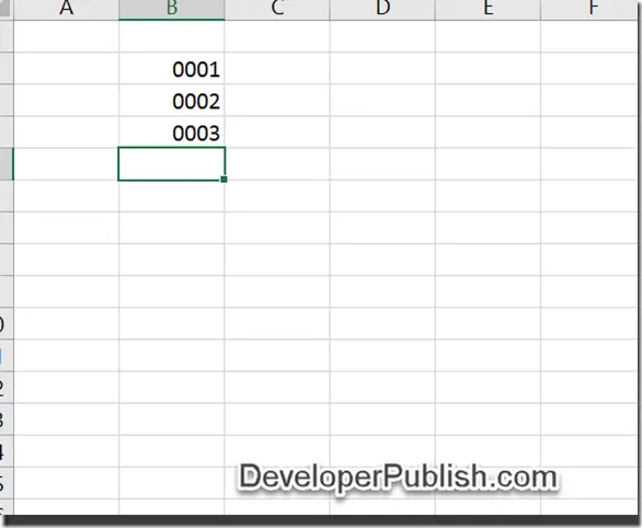
4. Now , when you type the value “1” in the cell and press the enter key , it should display it as 0001.

